Introduction
Pipe-to-soil potential changes caused by time varying dc interference are difficult to evaluate. The standards and guidelines usually refer to an acceptable pipe-to-soil potential range to determine if the pipe is cathodically protected and there is no risk of external corrosion. These values might typically be between -0.85 V and -1.2 V.
The question is what do you do when the potentials are varying outside these limits? Interference from dc traction systems can result in pipe-to-soil potentials outside of the acceptable limits.
Site Measurements
One method to evaluate the measured potentials is to use a datalogger to record the potentials over a period that provides data over the busiest times with the highest current loads. For dc traction systems this could be during a weekday rush hour. Practically speaking the dataloggers are usually placed for at least 24 hours, preferably longer, and with a sampling frequency of 0.5 s or 1 s.
Q Method - Analysis Methodology
The Q method is an established procedure for evaluating the time varying potentials and empirical guidelines have been developed to allow a judgement of the corrosion risk caused by the interference.
The method can be used to evaluate current densities as well as potentials. This example will deal with the potentials, but the principles are the same.
Q Method - Step by Step
Step 1 - Eref
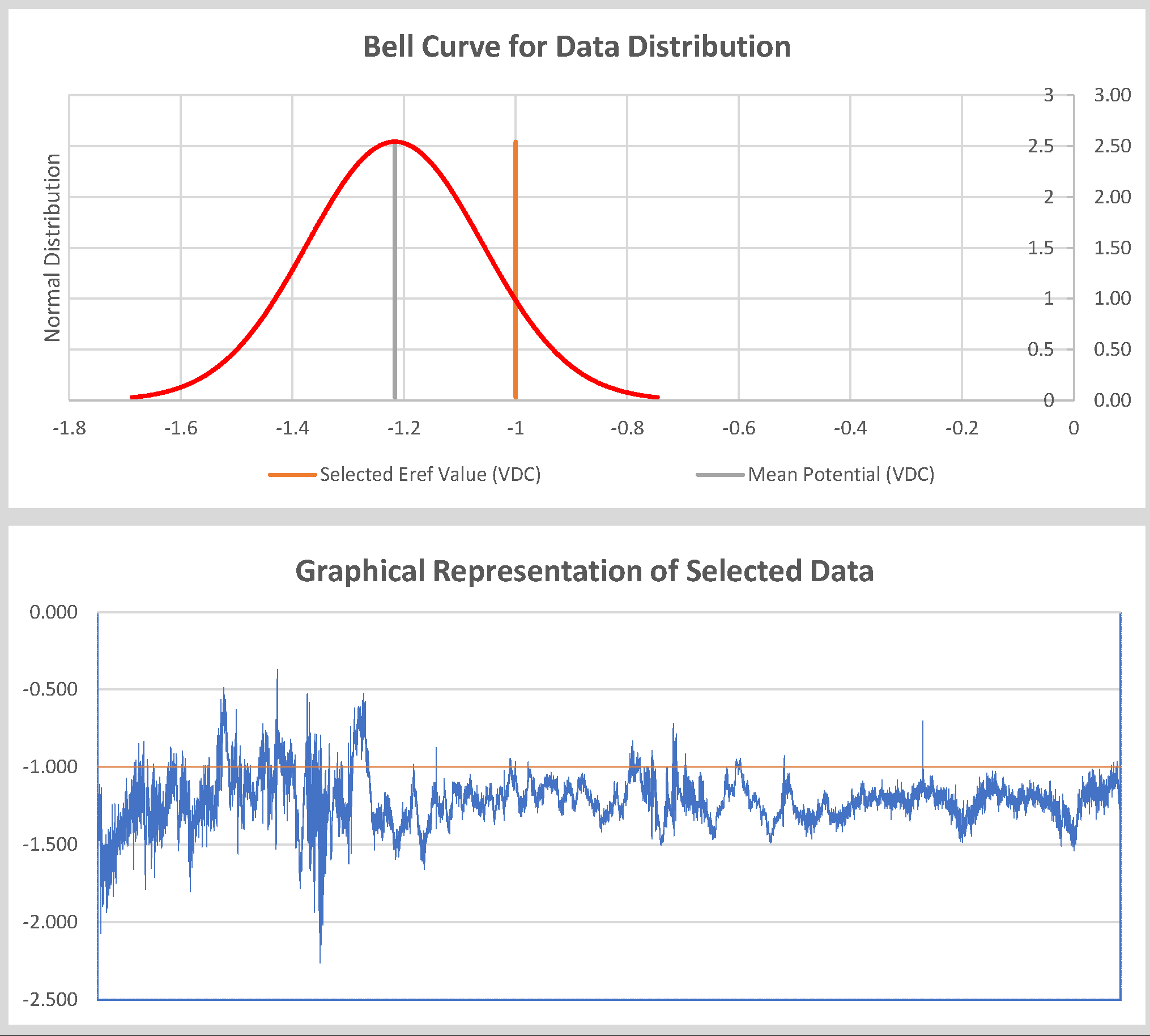
Select your reference potential. This is the value that you consider represents the protection potential you require for your pipeline. A typical value would be -1 V.
Step 2 - Tc
Establish the periods when the potential is more negative than the reference potential to give you the cathodic interval.
Step 3 - Ta
Establish the periods when it is more positive than the reference potential to give you the anodic interval.
Step 4 - Eon,avg
Calculate the average on potential by adding up all the potentials and dividing by the total number of measurements.
Step 5 - E’
Subtract the reference potential (Step 1) from all the measurements and replace all negative values with 0.
Step 6 - Ea,avg
Take the average of all the measurements of Step 5, add them up, and divide by the number of measurements. This gives the anodic average.
Step 7 - E’’
Subtract the reference potential (Step 1) from all the measurements and replace all positive values with 0.
Step 8 - Ec.avg
Take the average of all the measurements of Step 7, add them up, and divide by the number of measurements. This gives the cathodic average.
Step 9 - Ta,max
Establish the longest period of continuous anodic interference interval in seconds.
From this information it is possible to determine the Q factor (ratio) between the anodic and cathodic periods.
Notes
To evaluate the Q factor it is necessary to calculate the acceptance Factor.
If the Q value is greater than the Factor then protection against stray current corrosion has been achieved.
A fuller explanation is provided in the ISO standard 21857, which is presently under preparation.
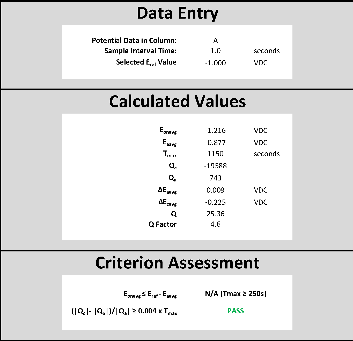
Evaluation Spreadsheet - DC Stray Current
To assist with validation of the software you use to carry out the Q factor calculations you can use the Corroconsult spreadsheet - Downloadable from the button at the end of this post.
You can also add your own data to perform the analysis, just be sure to “Clear Contents” of any previous data cells on the first tab [Paste Raw Data Here] - DO NOT Delete Columns / Rows as the calculation will not function.
Measurement interval, including fractions of a second, the data column that you wish to analyse and the Reference Value can all be specified in the second tab [Input & report].
The spreadsheet has been validated by Mathcad and Matlab calculations (available upon request).